Fourier Transform Definition, Visualisation & MATLAB Code (Steve Blog Ref)

Definitions of Fourier Transform:

The time domain (or spatial domain for image processing) and the frequency domain are both continuous, infinite domains. There is no explicit or implied periodicity in either domain. This is the one I call the Fourier transform.
The time domain is continuous and the time-domain functions are periodic. The frequency domain is discrete. I call this the Fourier series.
The time domain is discrete and infinite, and the frequency domain is continuous. In the frequency domain the transform is periodic. This is the discrete-time Fourier transform (DTFT).
The time domain and the frequency domain are both discrete and finite. Although finite, the time and frequency domains are both implicitly periodic. This form is the discrete Fourier transform (DFT).

Fourier Visualization:

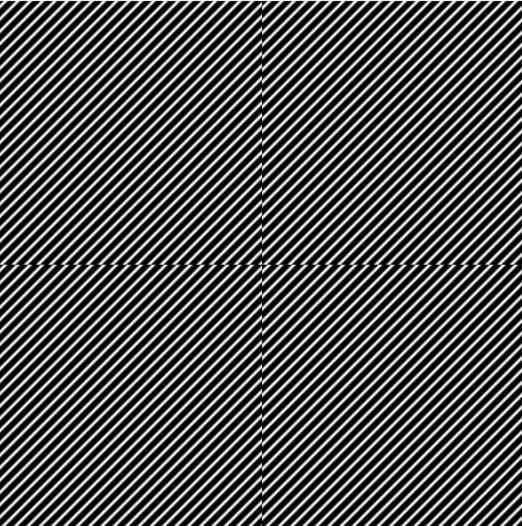
Here is the first example, the input image contains the single sinusoidal pattern, while doing 2D Discrete Fourier Transform it can be seen that the output contains slanting line which actually contributes to the image energy along with some vertical and horizontal lines. The reason can be understood by replicating the first picture as shown and you can easily see the discontinuity in the edges (horizontal and vertical lines). This discontinuity has broad range of energy in various frequency bands and thus contributing to straight vertical and horizontal lines. This effect can be removed by tapering the boundaries with zeros intensity values. The output of the Fourier transform after tapering is shown in the last figure.

MATLAB CODE:

url = 'http://blogs.mathworks.com/images/steve/2009/lines.png';

f = imread(url);

imshow(f)

F = fft2(f); %2D Discrete Fourier Transform using Fast fourier transform method

imshow(log(abs(fftshift(F)) + 1), []) %To plot the output

I4 = repmat(I, 2, 2); %to repeat the image

imshow(I4)

[M, N] = size(f);

w1 = cos(linspace(-pi/2, pi/2, M)); %Tapering the Edges

w2 = cos(linspace(-pi/2, pi/2, N));

w = w1' * w2;

f2 = im2uint8(im2single(f) .* w);

imshow(f2)

Comments

Digital Half Toning - Ordered Dithering - MATLAB Code Bayer/ Ulichney

Digital Half-toning is a technique to convert the gray scale / color image (in the range 0-255) to binary images (in the range 0-1) that is useful for printing (especially black and white printers). Though at first glance dots are clearly visible, as Human Vision System is a low pass filter, when dots are printed closely and viewed from the specific distance it can be perceived as a continuous tone image (i.e. gray scale). In general, half toning techniques is widely used in newspapers, journals and magazines printing. Halftoning algorithms aims for better #Image Quality #Low Complexity #Optimal ink usage Coming to the topic, Ordered dithering is one of the standard technique to produce halftone image from continuous (gray scale) images. Let us assume, the first block containing 'B' is an image matrix and the 'H' is the threshold matrix. And the process is simply a element wise (pixel wise) comparison; if element of B > H (g...

Digital Half-toning Error Diffusion Method (Floyd-Steinberg) - MATLAB Code

Introduction to Digital Half toning is provided in the below link http://imageprocessing-sankarsrin.blogspot.tw/2016/12/digital-half-toning-ordered-dithering.html The halftones are generally obtained by thresholding each image pixel with a certain value (ex. 128). In error diffusion, the error is computed between the actual and obtained output and it is distributed to the neighborhood pixels. Floyd-Stein berg, Jarvis, Stucki kernels are widely adopted to distribute the error. The Error Diffusion half toning is as follows 1) image(x,y) > 128 Apply thresholding (assume the image pixel value is 157, in that case, 255 will be assigned to output). ( as the half toning corresponds to two values 0 and 255) 2) Compute the error between actual and obtained output E= 255-157= 98 3) In case of floyd steinberg the value 98 is distributed along the neighborhood pixels 4) This steps are performed in sequence and serpentine scan yield...

Direct Binary Search Halftoning (DBS) - MATLAB Code (Efficient Direct Binary Search, Halftoning)

Direct binary approach is a heuristic optimization method and is proven to be very powerful to obtain optimized binary patterns. The approach achieves the least minimum square error between the perceived halftone and original image, though swap and toggle operation. The swap operation consists of switching the current pixel with eight of its neighborhood pixels. Toggle operation is about switching the values between 0 to 1 or vice versa (as shown in Fig. below) With each iteration, the perceived error starts to reduce and in finally a superior halftone quality is achieved. The method is computationally very expensive and difficult to implement in hardware. The code for Efficient DBS is provided in the link: (MATLAB Code) https://github.com/SankarSrin/EDBS-Halftoning

Image Processing (Digital Halftoning, Compression, ML & DL Models)

Search This Blog